How to choose the right imaging approach based on time, intent, and sky conditions

Introduction

Not every object requires long integration. The time involved in an astrophotography project depends on a range of factors: target distance, size, and brightness; your Bortle scale and local sky conditions. You’ll also need to consider your mount’s tracking and guiding capabilities, and the optical speed of your imaging system.
These variables influence not only how long you need to capture data, but also how you might configure your optical train; such as adding a reducer to widen your field of view and accelerate your f-ratio. But that’s only part of the story. In many cases, your ability to go deep may simply be limited by your schedule, weather, or travel constraints.
Much of this knowledge comes not from tutorials or specs, but from direct experience. You learn how your gear behaves as a system under your skies, and when it’s worth chasing depth versus maximizing speed.

That’s exactly what we’ll explore here, starting with:

What Does “Going Fast” Mean?

In astrophotography, “fast” refers to your imaging system’s focal ratio, or f-ratio. This is calculated by dividing the focal length of your telescope by the diameter of its aperture. The result is a dimensionless number, like f/2.8 or f/7, that tells you how quickly your system collects light. A lower f-ratio means a faster system, because the light is more concentrated on the sensor. In practice, an f/4 setup will gather the same signal four times faster than an f/8 setup.

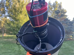
f = FL / D

This image is of my HyperAF system, a DIY f/1.9 imaging system which replaces the secondary mirror on my Celestron EdgeHD 8. By removing the secondary and replacing with the HyperAF image train, I effectively reduce my focal length to 388 mm. The result is a wide field of view with exceptionally high light gathering capability. Check out my article on The Fastest Imaging Rig I’ve Ever Built!

Fast systems typically provide wide fields of view and are well-suited for shorter exposure times. These setups are ideal for limited time sessions such as a weekend trip to a dark site where you only have one or two nights to gather as much data as possible. The goal of this configuration is to maximize signal acquisition per minute of exposure. Fast imaging is also a good fit for mosaics, wide-field surveys, or capturing bright broadband targets like galaxies and star clusters.

Going fast doesn’t mean cutting corners, it means knowing how to extract the best possible result from the time and conditions available to you in a field of view that meets your compositional intent. However, sometimes the goal isn’t to collect data quickly. The goal may be to reveal the delicate complexity hidden in the dimmest parts of a target. Going deep is a deliberate approach that prioritizes patience, layering, and refinement over time. While low f-ratios help maximize signal acquisition, resolving fine detail often depends more on focal length and image scale. Deep integrations not only improve signal-to-noise, but also unlock subtle structure, tonal gradients, and greater compositional control that short, wide-field sessions may miss.

What Does “Going Deep” Mean?

Going deep in astrophotography means committing to long integration times to push your signal-to-noise ratio as far as possible. This often involves using higher focal ratios, typically f/6 or above, and longer focal lengths that provide greater resolution. Deep imaging sessions are commonly spread over multiple nights, allowing for stacked data that reveals subtle structure and faint background features.

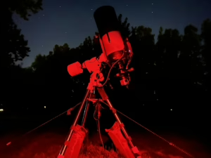
In this image is my Celestron EdgeHD 8 in 1422mm focal length configuration with .7x reducer. When setup in this configuration the scope is running at f/7, probably my favorite configuration. While it does sacrifice the speed of the f/1.9 configuration, it gains in detail, guiding stability, focus precision, and deep detail of distant, dim, objects.

This approach excels when targeting low-surface-brightness objects or complex detail: the outer shells of planetary nebulae, faint dust in galaxies, or extended emission regions in nebulae. These subjects benefit from accumulated signal, compositional consistency, and refined calibration practices. Subtle gradients and structural transitions often require high dynamic range and careful processing, both of which improve dramatically with longer integrations. Without sufficient depth, these details may remain hidden beneath the noise floor, never fully realized in the final image.

Going deep isn’t about one type of gear or one kind of image. It’s about patience, stability, and intent. It’s a deliberate choice to prioritize detail, depth, and tonal nuance over quick capture or broad coverage. Regardless of whether you’re going fast or deep, calibration is the foundation that makes clean, accurate data possible. Understanding how often to capture different types of calibration frames—and how they apply across single or multi-night sessions—is essential to every imaging strategy.

The Calibration Consideration

Calibration is critical no matter your imaging approach. Fast or deep, the quality of your final image depends on how well you’ve addressed the inherent noise and imperfections of your system. The only calibration frame that truly must be taken during each imaging session is flats. These are highly sensitive to changes in filter, focus, and rotation, and must be recaptured whenever your optical configuration changes. All other calibration frames—darks, bias, and dark flats—can be reused from a master library, provided they match your camera’s settings such as temperature, gain, binning, and exposure length. These master frames can remain valid for months at a time.

A common misconception is that multi-night imaging is harder to calibrate. In reality, with good calibration discipline and an organized master library, stitching together data from multiple nights is just as straightforward as processing a single session. If you want to get serious about your calibration strategy—whether you’re optimizing for speed or building up deep integrations—check out An Astrophotographer’s Field Guide to Calibration Frames. It’s built from the ground up to support workflows like the ones featured here on AstroAF.

Quick Reference: Calibration Frame Essentials

Calibration Type	Cover	Exposure	Temp	Gain	Bin	Notes
Darks	On	Match lights	Match lights	Match lights	Match lights	Captures thermal signal. Can be reused as a library.
Bias	On	Shortest possible	Match lights	Match lights	Match lights	Captures read noise. Can be reused as a library.
Flats	Off	1–4 sec typical	Match lights	Match lights	Match lights	Captures system specific artifacts
Dark Flats	On	Match flats	Match flats	Match flats	Match flats	Used instead of Bias. Captures thermal signal. Can be reused as a library.

Bonus Calibration Diagram

Here’s a different type of visualization of the Quick Reference that you can download and keep handy for reference.

When to Choose Each Approach

When you might go fast:
You’re imaging a large target that demands a wide field of view.
Some objects, like the North America Nebula, Rosette, Andromeda Galaxy, or the full Moon don’t fit in a narrow field. In these cases, you have to go wide, which naturally leads to faster optics and shorter focal lengths.

Fast systems are a natural fit when you’re aiming for broad compositions and efficient data capture.
Fast systems, like f/2–f/4, gather light efficiently, making them ideal for capturing large swaths of the sky in less time. They’re great for surveys, Milky Way fields, and targets that benefit from a broad frame.

You’re imaging bright targets that respond well to short exposures.
Many widefield subjects, like emission nebulae and major galaxies, are relatively bright and structured, meaning even short subs can pull out compelling detail at fast f-ratios.

You’re running a simple, lightweight, mobile rig, no guiding, fast exposures, minimal gear
This type of rig is perfect for quick setup and teardown, skipping the complexity of guiding, and simply shooting short exposures with just a tracker and camera. This approach minimizes gear while maximizing flexibility, especially when traveling or dodging clouds.

You’re at a dark site for just 1–2 nights.
With limited time under quality skies, going fast allows you to maximize your dataset and walk away with a complete image. Instead of spreading thin across multiple nights, you can focus your effort and return with a finished result, even from a single session.

Skies are changing or conditions are marginal.
When conditions aren’t perfect, faster setups and shorter exposures let you adapt quickly. Whether you’re working in between clouds, dealing with poor seeing, or working around moonlight; you can walk away with a solid image when the night isn’t ideal.

You might go deep when:
You’re aiming for a narrower, zoomed-in field of view that highlights structure and detail within a specific region of a target. This typically calls for a longer focal length and slower f-ratio system, which increases magnification and resolution at the expense of speed.

You want to capture subtle, intricate features such as faint wisps of nebulae, shock fronts, or fine galactic dust lanes that only emerge with higher signal-to-noise from long integrations.

You’re not limited to a single night of data. Whether you’re working from a permanent setup, imaging from home, or have repeatable framing across sessions, stacking data over multiple nights allows you to push much deeper.

You’re deliberately averaging sky conditions across sessions. By integrating under varying transparency and seeing, you gain flexibility in scheduling and can build toward a result that exceeds what’s possible on any single night alone.

You’re targeting dim or diffuse subjects like integrated flux nebulae, dark nebulae, or supernova remnants that demand hours or even tens of hours to reveal properly.

Real-World Examples

• Fast Integration:
• 
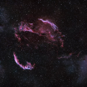
  This is a 9 Panel Mosaic of the Cygnus Loop (Veil Nebula Complex) from only 8 1/2 hours of subframe integration using my HyperAF system at f/1.9.
  Cygnus Loop (Veil Nebula Complex) is a gigantic supernova remnant in the constellation Cygnus. The arcs of the loop are known collectively as the Veil Nebula. The Cygnus Loop is located 1470 Light Years From Earth.

About this image:

9 Panel Mosaic
Unguided 28 x 120 sec Subframes Per Panel
08:38 Hours Total Integration

Acquisition Gear:

Celestron EdgeHD 8 In “HyperAF” Configuration f/1.9 | 388mm
ZWO Astrophotography ASI533MC Pro
Optolong Astronomy Filter Ha/Oiii Duo-Narrowband
Astroasis Oasis Focuser
Sky-Watcher USA HEQ5 Pro

Software:

Captured in NINA
Processed in Pixinsight

Deep Integration:

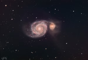
This image is Messier 51, discovered by Charles Messier in 1773. Its striking spiral structure was later revealed by Lord Rosse in 1845, making it the first galaxy identified as having a spiral form. M51’s interaction with its companion galaxy has made it a key object of study in galactic dynamics.

Common Name: Whirlpool Galaxy
Type: Grand-Design Spiral Galaxy
Constellation: Canes Venatici
Apparent Magnitude: 8.4
Angular Size: 11.2 × 6.9 Arcminutes
Coordinates (J2000): RA 13h 29m 52.7s | Dec +47° 11′ 43″
Approximate Distance from Earth: 31 Million Light-Years
Companion Galaxy: NGC 5195

Image Information:

Total Integration: 43h 10m
2332 mm Bin 2
L 104 x 300
R 53 x 300
G 53 x 300
B 53 x 300
Sii 30 x 900
Ha 28 x 900
Oiii 27 x 900

Equipment Used:

Celestron EdgeHD 8
​⁠Player One Astronomy Artemis-M Pro
​⁠Optolong Astronomy Filter LRGB
​Svbony Filter SHO
​Astroasis Oasis Focuser and Filter Wheel​⁠
Sky-Watcher USA HEQ5 Pro

Software:

Captured in NINA
Processed in Pixinsight

How Signal-to-Noise Changes Over Time

Signal in an image increases linearly with exposure time, double the exposure and you double the signal collected from your target. But noise behaves differently. While some types of noise (like thermal or read noise) may accumulate, random noise from the sky background and your electronics tends to average out the more you expose and stack.

This is where the inverse square relationship comes into play.

The Math Behind It:

As you capture more total exposure time, your signal increases linearly and each subframe adds more photons from your target. But the noise decreases more slowly. In fact, the improvement in signal-to-noise ratio (SNR) follows an inverse square relationship with respect to noise.

The math behind this is simple:

SNR ∝ √T

Where:
SNR (signal-to-noise ratio)
Is proportional to
The Square Root of T (the total integration time)

SNR improves proportionally to the square root of total exposure time. So if you increase your total integration time by 4x, your SNR only improves by 2x. To double your SNR, you need to capture four times as much data.

This diminishing return is important in practice. For example, Going from 1 hour to 4 hours doubles your SNR but going from 4 hours to 8 hours only gives you a ~41% gain. The first few hours make a big difference, each extra hour helps but not as dramatically as the first. That’s why deep imaging takes patience. Every additional hour makes the image cleaner, but with diminishing returns, especially if your skies aren’t ideal. Persistence pays dividends.

Diminishing Returns and Knowing When to Stop

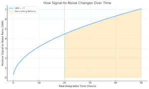
While signal-to-noise ratio improves with more data, the rate of improvement slows over time. Because SNR increases with the square root of total exposure, doubling your integration time doesn’t double your quality, it gives you only a modest boost. Eventually, you’ll hit a point of diminishing returns where the effort to gather more frames yields only subtle improvements. There’s no universal rule for when to stop. SNR estimation tools can give you a general sense of progress, but they shouldn’t make the final decision for you. The best practice is to monitor your own data: create trial integrations along the way, inspect the results, and let your eye and your goals be the guide. Trust your judgment, you will know when you are happy with your data.

This chart is illustrating the square root relationship between integration time and signal-to-noise ratio (SNR). The shaded region which starts around 20 hours represents where diminishing returns begin. This is just an illustrative example and does not represent your own data conditions. This chart is purely intended as a data scenario example to help explain diminishing returns.

Final Thoughts

• Every imaging session is a balance between opportunity and intention. If you are curious about what I mean by intention then check out my post on Astrophotography With Intent. Whether you’re chasing photons under fleeting skies or building a masterpiece over many nights, the approach you choose should reflect your goals, your conditions, and what excites you about the target.
• There’s no one-size-fits-all. Sometimes it’s about capturing something meaningful in a single night. Other times it’s about digging deeper and watching an image take shape over weeks. Both are valid, rewarding, and worth celebrating.
• Trust your judgment, adapt when needed, and most of all, enjoy the process.

Cheers!
Doug

Join AstroAF on YouTube
Join AstroAF on Buy Me a Coffee
Join my Discord Server