What Is a Palette?

In astrophotography, a palette refers to the method by which an imager assigns individual data channels to the red, green, and blue components of a final color image. These channels can originate from broadband filters that approximate visible light, or from narrowband filters that isolate specific emission lines within the visible spectrum. Regardless of the source, the palette determines how those channels are blended to create an image that is both scientifically meaningful and aesthetically pleasing. For broadband imaging, the palette is generally fixed because the data corresponds directly to the red, green, and blue wavelengths captured by the sensor. Red data maps to red, green to green, and blue to blue, creating a representation that closely resembles what the human eye would perceive if it were sensitive enough to detect faint astronomical objects. This convention provides consistency and an intuitive connection between the data and the final image.

In narrowband imaging, however, the imager collects light from very specific emission lines — such as sulfur-II (SII) at approximately 672 nm, hydrogen-alpha (Ha) at approximately 656 nm, and oxygen-III (OIII) at approximately 501 nm — each of which represents a narrow slice of the visible spectrum. When using a monochrome camera, the photographer captures each of these channels separately through dedicated filters, resulting in individual grayscale images. These separate images must then be assigned to the red, green, and blue channels during post-processing, which introduces the creative and technical choice of which palette to apply. Conversely, a one-shot color (OSC) camera captures all three broadband color channels simultaneously using a Bayer matrix. Although it is possible to use narrowband filters with an OSC camera, the process is more restrictive because the camera combines the color information at the time of capture. This limitation reduces the flexibility in mapping narrowband data into a palette, making monochrome cameras generally preferred for constructing advanced and custom palettes.

The most common palette used in narrowband imaging is the Hubble Palette (SHO). In this mapping, SII is assigned to red, Ha to green, and OIII to blue, producing the iconic gold-and-blue images popularized by NASA’s Hubble Space Telescope. However, the SHO palette is just one of many possibilities. Other palettes, such as HSO, HOO, and FORAX, explore alternative assignments to emphasize different structures, enhance contrast, or simply create a more visually appealing image. One of these alternative palettes is called FORAX, which blends the same SII, Ha, and OIII data but with weights chosen to enhance balance and color richness beyond what SHO provides. The FORAX palette produces a nuanced, customizable image that many imagers find more satisfying, both technically and artistically. This post will explain what FORAX is, describe its formula, and share why I selected it for my M27 project, along with a brief overview of how to apply it to your own work.

Common Narrowband Palette Reference

Palette	Red Channel	Green Channel	Blue Channel
SHO (Hubble)	SII	Ha	OIII
HSO	Ha	SII	OIII
HOO	Ha	OIII	OIII
OHS	OIII	Ha	SII
Bicolor (Ha/OIII)	Ha	Ha + OIII	OIII

Astrophotographers can think of a palette as a recipe: it allows them to assign specific data to each color channel in order to showcase the distinct physical processes traced by each emission line, as well as the spatial distribution of elements revealed by the filters. For example, mapping sulfur-II emphasizes cooler, outer regions of ionized gas; hydrogen-alpha highlights regions of active star formation and dense ionized hydrogen; and oxygen-III brings out hotter, high-energy zones often associated with shock fronts and stellar winds. By choosing how these channels are combined, imagers can both convey scientific information and achieve their preferred aesthetic.

Why SHO? Why Alternatives?

One of the most widely used palettes in narrowband astrophotography is the Hubble Palette (SHO), named for its association with the Hubble Space Telescope. In this mapping, sulfur-II (SII) data is assigned to the red channel, hydrogen-alpha (Ha) to the green channel, and oxygen-III (OIII) to the blue channel. The SHO palette has become a standard because it produces the distinctive gold-and-blue images that many people now associate with nebulae, and it also provides a meaningful way to visualize the relative contributions of these three emission lines in a scientifically recognizable form (Hester et al., 1996; HubbleSite, 2010).

The Hubble team developed the SHO palette in the mid-1990s when imaging the Eagle Nebula (M16) and other objects through narrowband filters. They faced a challenge: both SII and Ha occupy similar red wavelengths and would overlap if mapped “naturally,” leaving little visual distinction between them. To solve this, they assigned each emission line to a different primary color channel in a way that maximized contrast and clarity. This approach, known as representative color, allowed viewers to easily discern the physical structure traced by each element while also creating a visually engaging image (HubbleSite, 2010). Although the palette’s striking aesthetic contributed to its popularity, the primary motivation was to produce an image that was scientifically meaningful, interpretable, and educational for a broad audience (Hester et al., 1996).

However, while the SHO palette is iconic, it is not without limitations. Many imagers find that the strong green contribution from Ha can overwhelm subtle details, producing unnaturally vivid green tones in some nebulae. Others observe that the balance between the red, green, and blue channels in SHO does not always reflect the physical contrasts they wish to emphasize, particularly in objects with highly uneven signal strengths across the channels. Additionally, the rigid one-to-one assignment of each emission line to a single color channel limits creative flexibility and can make star fields appear harsh or unnatural.

As a result, many astrophotographers explore alternative palettes that adjust these assignments and weights to highlight specific features of the target or achieve a more pleasing aesthetic. Palettes such as HSO, HOO, and OHS reassign the same SII, Ha, and OIII data into different color channels, allowing imagers to suppress unwanted tones, enhance particular filaments or shock structures, or create more natural-looking stars. The FORAX palette is one such alternative, designed to provide a balanced, tunable color representation that many find more satisfying, both scientifically and artistically, than the traditional SHO.

What Is FORAX?

The FORAX palette was developed by astrophotographer Maxime Oudoux, who began sharing the technique with the astrophotography community around 2018 under his online pseudonym FORAX. This alias was the name he used on astrophotography forums and galleries when presenting his work. Although some have speculated that FORAX is derived by reversing or rearranging his real name, there is no clear linguistic connection between “Maxime Oudoux” and “FORAX.” Rather, it appears to have been simply a distinctive and memorable handle that became associated with his palette in the astrophotography community.

The FORAX palette is a custom mapping of narrowband data that rebalances the contributions of sulfur-II (SII), hydrogen-alpha (Ha), and oxygen-III (OIII) to produce an image that is both scientifically meaningful and aesthetically pleasing. While the Hubble Palette (SHO) assigns each emission line exclusively to one color channel, FORAX introduces weighted combinations of channels to achieve more subtle, controlled color transitions and to reduce overpowering tones often present in SHO images.

At its core, FORAX blends the SII, Ha, and OIII data into the red, green, and blue channels using tunable weights. Instead of mapping SII strictly to red, Ha strictly to green, and OIII strictly to blue, FORAX distributes the signal so that each channel benefits from contributions of multiple emission lines. This results in smoother gradients, more balanced star fields, and better separation of faint structures.

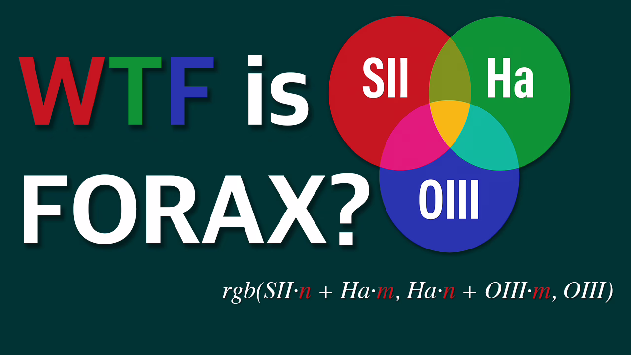
The general formula for FORAX can be written symbolically as:

rgb(SII·n + Ha·m, Ha·n + OIII·m, OIII)

where:

• SII, Ha, and Oiii are the monochrome masters for each emission line.
• n and m are weighting coefficients that you can adjust to taste, typically with n>m to favor the primary contributor in each channel.

For example, a commonly used set of weights might set n to 0.8 and m to 0.2, resulting in:

rgb(SII·0.8 + Ha·0.2, Ha·0.8 + OIII·0.2, OIII)

However, one of the advantages of FORAX is its flexibility — these weights are not fixed, and imagers can adjust them depending on the characteristics of their data and the look they wish to achieve. This tunability allows FORAX to address some of the criticisms of SHO, such as excessive green or muted reds, while still clearly distinguishing the physical processes traced by each emission line.

In the next section, I will demonstrate how to apply FORAX in practice, starting from calibrated master frames and preparing them for combination in PixelMath to create a final RGB image ready for further processing.

Applying FORAX: From Masters to RGB

With the concept of the FORAX palette defined, the next step is to apply it to real data. In this section, I will walk through my own workflow for preparing calibrated master frames and combining them into a single RGB image using the FORAX formula. This is not the only way to approach it, but it is a reliable and repeatable process that produces excellent results.

Step 1: Calibrated Masters from WBPP

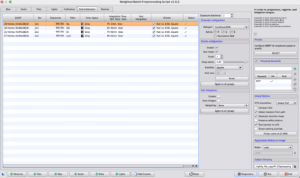
Produces a set of clean, linear master frames for each of your narrowband filters — typically sulfur-II (SII), hydrogen-alpha (Ha), and oxygen-III (OIII). These masters are the starting point for the rest of the workflow. They are shown here in the Preprocessing tab of the WeightedBatchPreProcessing process window which provides the post-calibrated results to expect from the final stacked integration.

Step 2: Apply Dynamic Crop

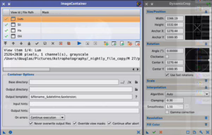
Once I have the master frames, I use DynamicCrop to remove any stacking artifacts or mismatched field edges. To ensure all masters are cropped identically, I set up the crop on one channel and then drag the process icon into the Process Console gutter to save it. I then apply the same saved crop to an image container which applies the crop to all images in the same step. This keeps all the data perfectly aligned and leaves me with clean, matched frames. I save the custom crop to an icon in case I need to reuse it later.

Step 3: Background Extraction

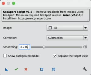
With the cropped masters, I remove any residual background gradients using background extraction. In this particular dataset, I tested several methods — Seti Astro’s Automatic DBE script, PixInsight’s native DBE and ABE, and GraXpert Background Extraction from the toolbox (Script > Toolbox > Graxpert). For this particular data, GraXpert delivered the most natural-looking result, so I used it. I recommend trying a few options and choosing the one that best suits your specific data, as the optimal method can vary. Background extraction is one of the most critical steps that can impact how your downstream processing steps will go. Take your time here and keep after it until you get the result you expect. I like to run this on each image individually and then inspect, however, this can be run directly on the image container if you wish.

Step 4: Noise Reduction

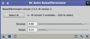
Next, I reduce noise in the linear masters using NoiseXTerminator. At this stage, we are still working with linear images, and running noise reduction now helps maintain faint details while taming background noise. Normally, just the default settings are appropriate at this stage of processing. This can be run upon the image container if desired. With that said, make sure an inspect your images after the application of noise reduction, especially for the following:

Mottling — Patchy, blotchy, uneven texture in the background of an image, often after noise reduction or stretching. It refers to random, irregular spots and patterns in what should otherwise be a smooth area.

Modeling — Sometimes used to refer to visible structures in the background (gradients or patterns) that reflect an incorrect model of the background, i.e., residual signal or gradients left uncorrected.

Step 5: Star Removal

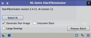
After noise reduction, I separate the stars from the nebula by running StarXTerminator on each master, you can also run this on the image container. This produces both a starless image and a separate stars-only image for each channel. I save the stars-only images to the Process Console gutter for later, as they will not be combined yet but may be reintroduced after post-processing.

Step 6: Histogram Transformation

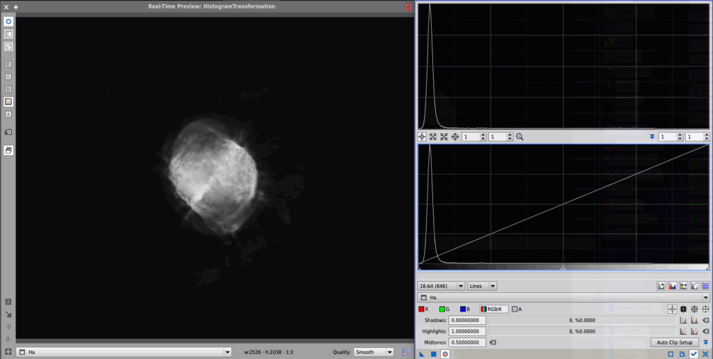
With the cropped, gradient-corrected, noise-reduced, and starless masters prepared, I stretch them from linear to non-linear using HistogramTransformation. At this point you now have clean, stretched SII, Ha, and OIII masters ready to be combined. I suggest that you do not over-stretch the individual frames at this point, rather, leave some headroom for post-processing work in Curves Transformation. You will have plenty of opportunities to gradually boost signal and contrast along the way through your processing steps. It is best not to try and do it all in one step.

Step 7: Apply FORAX PixelMath

Finally, I use PixelMath to combine the three stretched masters into a single RGB image using the FORAX formula. The following is shown as a single RGB expression but you can just as easily split this into separate channels in pixelmath if you prefer.

rgb(SII·n + Ha·m, Ha·n + OIII·m, OIII)

where n and m are weighting coefficients that you can adjust to taste — for example, n = 0.8 and m = 0.2. In the PixelMath dialog, paste the formula into the RGB/K expression field, set the output to RGB color, and run the process. You now have an RGB image in the FORAX palette.

In this particular case, I also blended the result with my luminance master to improve contrast and enhance faint structural details. I did this by applying a second PixelMath expression of the form:

FORAX × ~(k – Lum)

where k is a small scaling factor — in my example, approximately k = 0.6 — that controls the strength of the luminance contribution. This adjustment preserves the FORAX color mapping while adding subtle texture and depth from the luminance channel.

Processing Summary and Final Adjustments

With the FORAX RGB image (and optional luminance blend) completed, the final stage of processing focuses on refining the image’s contrast, color balance, and overall aesthetic. These steps are performed on the combined RGB image and can vary depending on the data and artistic intent, but the following sequence is a solid starting point.

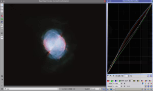
First, I use CurvesTransformation to adjust the brightness, contrast, and individual color channels. This step allows for precise tuning of the midtones and highlights while preserving faint structures. If needed, I also make small histogram tweaks at this stage to fine-tune the black and white points and improve dynamic range.

Next, I may apply a light color saturation boost to enhance the richness of the nebula and make subtle hues more visible. Finally, I adjust the image’s final contrast and black point using a simple but powerful expression in PixelMath:

$T × (1 - (1 - $T)^2.2 × 0.3)

This equation helps darken the shadows slightly while maintaining smooth transitions and preserving detail in the midtones and highlights.

What Does This Equation Do?

Let’s break it down:

• $T: This represents the current pixel intensity of the image.
• (1 - $T): This inverts the intensity, so dark pixels become light and vice versa.
• (1 - $T)^2.2: This applies a gamma-like curve to the inverted intensity, giving more weight to darker pixels while leaving brighter areas less affected. The exponent 2.2 controls the steepness of the curve.
• × 0.3: This scales the adjustment so it doesn’t overpower the image — blending just 30% of the effect.
• 1 - (...): This inverts the result back into the correct orientation.
• $T × (...): Finally, the original image is multiplied by this adjustment factor, subtly compressing the shadows and enhancing contrast in a controlled way.

The result is a gentle darkening of the darkest tones, improved separation between faint structures and the background, and a more polished, high-contrast look without harsh clipping.

Closing Thoughts

The FORAX palette is a powerful and flexible alternative to the classic SHO mapping, offering a more balanced and customizable way to present narrowband data. By carefully preparing your masters, applying thoughtful pre-processing, and combining the channels with tunable weights, you can create images that both honor the physical reality of the object and reflect your personal artistic vision. The ability to enhance your RGB result further with luminance blending and subtle contrast adjustments allows you to fine-tune the final image into something truly unique.

Whether you are a seasoned imager looking to try something new or a beginner exploring beyond SHO for the first time, the FORAX palette provides a creative and satisfying workflow. Like any technique in astrophotography, it rewards experimentation — adjust the weights, tweak your post-processing steps, and see how the palette brings your data to life.

If you found this guide helpful or have your own FORAX results to share, I’d love to see them. Leave a comment below, tag me on your favorite platform, or reach out through the contact links on my site. And if you’re interested in more walkthroughs, tips, and astrophotography guides, consider subscribing to the blog or joining the AstroAF community for more resources and discussion.

Clear skies, and happy imaging!

Cheers!
Doug

Join AstroAF on YouTube
Join AstroAF on Buy Me a Coffee
Join my Discord Server

Download The FORAX and Background Contrast Process Icons

References

Hester, J. J., Scowen, P. A., Sankrit, R., Lauer, T. R., Ajhar, E. A., Baum, W. A., … & Westphal, J. A. (1996). Hubble Space Telescope WFPC2 imaging of M16: Photoevaporation and emerging young stellar objects. The Astronomical Journal, 111(6), 2349–2360. https://doi.org/10.1086/117933

HubbleSite. (2010). Behind the pictures: Using color to explore the universe. Retrieved from https://hubblesite.org/resource-gallery/articles/2010-06-behind-the-pictures-using-color-to-explore-the-universe